How long will my machine last?

Applying Bayesian statistics to a manufacturing problem.

When writing about confidence intervals I came across this 1974 paper by E. T. Jaynes which had a nice problem about estimating the minimum lifetime of some machinery.

EXAMPLE 5. TRUNCATED EXPONENTIAL DISTRIBUTION

The following problem has occurred in several industrial quality control situations. A device will operate without failure for a time \(\theta\) because of a protective chemical inhibitor injected into it; but at time \(\theta\) the supply of this chemical is exhausted, and failures then commence, following the exponential failure law.

It is not feasible to observe the depletion of this inhibitor directly; one can observe only the resulting failures. From data on actual failure times, estimate the time \(\theta\) of guaranteed safe operation by a confidence interval. Here we have a continuous sample space, and we are to estimate a location parameter \(\theta\), from the sample values \({ x_1, x_2, \ldots x_n }\), distributed according to the law \[ p(dx \mid \theta) = \begin{cases} \exp(\theta - x) dx & x > \theta, \\ 0 & x < \theta . \end{cases} \]

I love this kind of “real life” problem. The paper makes the point that calculating a confidence interval is complicated and results in a completely unhelpful interval. It shows how a Bayesian approach gives much better results, but the paper jumps through to defining a posterior density without showing how it gets there. I wanted to work it though and thought it would be a chance to try out using Stan.

Some maths

Poisson processes can be used to model the number of events which occur over time – things like the number of phonecalls received in a call centre, the number of people who walk into a shop, or the number of cars which pass you by as you walk down the street.

If we denote the number of events to occur up to some time \(t\) as \(N(t)\), then the probability that \(N(t) = n\) is given by the Poisson distribution:

\[ P(N(t) = n) = \frac{(\lambda t)^n}{n!} e^{-\lambda t} \]

where \(\lambda\) is the rate of events per unit time.

In our example an event is the failure of a machine. We’re interested in the time of each failure which we label as \(T_1, T_2, \ldots, T_N\). Each of these times is independent of the others.

We can notice that the event \(T_1 > t\) is equivalent to saying that no events occurred by time \(t\), which is the same as saying \(N(t) = 0\). So we can write

\[ P(T_1 > t) = P(N(t) = 0) = e^{-\lambda t}. \]

Probabilities must sum to one, so we can also note

\[ P(T_1 \leq t) = 1 - P(T_1 > t) = 1 - e^{-\lambda t}. \]

The result, \(1 - e^{-\lambda t}\), is the cumulative distribution function for an exponential distribution with rate \(lambda\), with probability density function

\[ p(t \mid \lambda) = \lambda e^{-\lambda t}. \]

This means that \(T_1 \sim \text{Exponential}(\lambda)\). By using the memorylessness property of the exponential distribution we can say that all \(T_1, T_2, T_3\) etc. are exponentially distributed.

---

In our problem there’s an added constraint – the machines will run for a time \(\theta\) before the chemical inhibitor is exhausted and failures begin. This means that the failure times have a lower bound – they will be at least \(\theta\) – which leads us to describe the failure times as following a shifted exponential distribution

\[ p(t \mid \lambda, \theta) = \begin{cases} \lambda \exp(-\lambda (t - \theta)) & x \geq \theta, \\ 0 & x < \theta. \end{cases} \]

If we set \(\lambda = 1\) and multiply out the negative sign, this would be equivalent to the distribution given in the Jaynes paper.

We can see the effect of the shifting by plotting the probability density function for different values of \(\theta\):

x_length = 8;

viewof lambda = Inputs.range([0.1, 3], {
  label: tex`\text{lambda: }\lambda`,
  step: 0.1,
  value: 1,
});
viewof theta = Inputs.range([0, x_length], {
  label: tex`\text{theta: }\theta`,
  step: 0.1,
  value: 0,
});
viewof t = Inputs.range([0, x_length], {
  label: tex`\Pr(X \leq t): t`,
  step: 0.1,
  value: 3,
});

x = Array.from({ length: x_length * 100 + 1 }, (_, i) => i / 100);
y = x.map((x_i) => lambda * Math.exp(-lambda * (x_i - theta)));
coordinates = x.map((x_i, i) => {
  return { x: x_i, y: (x_i >= theta) * y[i] };
});

filteredCoordinates = coordinates.filter((coord) => coord.x <= t);

Plot.plot({
  x: { domain: [0, x_length] },
  marks: [
    Plot.lineY(coordinates, { x: "x", y: "y" }),
    // Add the stuff for the cumulative probability
    Plot.areaY(filteredCoordinates, {
      x: "x",
      y: "y",
      fill: "blue",
      fillOpacity: 0.5,
    }),
    Plot.lineY(filteredCoordinates, {
      x: "x",
      y: "y",
      stroke: "blue",
      strokeWidth: 4,
    }),
    Plot.ruleX([[t]]),
  ],
});

Modelling as a Bayesian problem

The Jaynes paper derives a 90% credible interval for \(\theta\). A 90% credible interval is a range of values where there’s a 90% chance that the actual value is within that range (a property which is not shared by confidence intervals!)

Our goal is to get a formula for the probability density of \(\theta\) by using the observed failure times, so we can derive an interval for \(\theta\).

The Jaynes paper derives the posterior probability density for \(\theta\) as

\[ p(\theta \mid x_1, x_2, \ldots x_N) = \begin{cases} N\exp(N(\theta - \min(t))), & \theta < \min(t), \\ 0, & \theta > \min(t). \end{cases} \]

We can derive this using Bayes’ theorem,

\[ p(\theta \mid t_1, t_2, \ldots t_N) = \frac{p(t_1, t_2, \ldots t_N \mid \theta)p(\theta)}{p(t_1, t_2, \ldots t_N)}. \]

We choose a flat prior for \(\theta\), such that \(p(\theta) \propto 1\) and set \(\lambda = 1\) throughout. Since \(p(\theta) \propto 1\) and \(p(t_1, t_2, \ldots t_N)\) doesn’t depend on \(\theta\), we drop them as constants, ending up with

\[ p(\theta \mid t_1, t_2, \ldots t_N) \propto p(t_1, t_2, \ldots t_N \mid \theta). \]

Using the independence of each failure time, we continue to simplify the expression:

\[ \begin{align} p(\theta \mid t_1, t_2, \ldots t_N) & \propto p(t_1, t_2, \ldots t_N \mid \theta) \\ &\propto \prod_{i=1}^{N} p(t_i \mid \theta) \\ &\propto \prod_{i=1}^{N} \exp{(\theta - t_i)} \cdot \mathbb{1} \{ t_i \geq \theta \} \end{align} \]

where \(\mathbb{1} \{ t_i \geq \theta \}\) is the indicator function which is one if \(t_i \geq \theta\) and zero otherwise. Continuing, we note that the union of the events \(\{ t_i \geq \theta \}\) is the same as the event \(\min(t) \geq \theta\):

\[ \begin{align} p(\theta \mid t_1, t_2, \ldots t_N) &\propto \prod_{i=1}^{N} \exp{(\theta - t_i)} \cdot \mathbb{1} \{ t_i \geq \theta \} \\ & \propto e^{N \theta} \cdot \mathbb{1} \{ \min(t) \geq \theta \}. \end{align} \]

To get a probability distribution for \(\theta\), we recall that probability distributions must integrate to one,

\[ \int_{-\infty}^{\infty} p(\theta \mid t_1, t_2, \ldots t_N) d\theta = 1. \]

We look to integrate our formula for \(p(\theta \mid t_1, t_2, \ldots t_N)\). We can use the result to form a probability density which integrates to one,

\[ \begin{align} \int_{-\infty}^{\infty} p(\theta \mid t_1, t_2, \ldots t_N) d\theta &= \int_{-\infty}^{\infty} e^{N \theta} \cdot \mathbb{1} \{\min(t) \geq \theta \} d\theta \\ &= \int_{-\infty}^{\min(t)} e^{N \theta} d\theta \\ &= \frac{\exp{(N\min(t))}}{N} . \end{align} \]

If we divide our formula \(e^{N \theta} \cdot \mathbb{1} \{\min(t) \geq \theta \}\) by \(\frac{\exp{(N\min(t))}}{N}\) we get a probability distribution for \(\theta\) which integrates to one,

\[ p(\theta \mid t_1, t_2, \ldots t_N) = \begin{cases} N\exp(N(\theta - \min(t))) & \text{if } \theta \leq \min(t), \\ 0 & \text{otherwise} \end{cases} \]

which is the posterior probability given in the paper.

Deriving a credible interval

The paper provides three observed values for failure times: \({t_1, t_2, t_3} = {12, 14, 16}\). From this it derives a 90% credible interval for \(\theta\) of \(11.23 < \theta < 12\); this is what we aim to reproduce.

The resulting formula we’re trying to solve is to find \(L\) and \(U\) such that

\[ \int_L^U p(\theta \mid t_1, t_2, t_3) = 0.9. \]

We know that \(\theta \leq \min(t)\) and want to find the shortest credible interval, which means targeting the interval over the area with the bulk of the probability density. Since most of the probability density is near \(\min(t)\), we set \(U = \min(t) = 12\). Substituting in everything else, we can solve for \(L\):

\[ \int_L^{12} 3\exp(3(\theta - 12)) = 0.9. \]

Let’s expand the integral:

\[ \begin{align} \int_L^{12} 3\exp(3(\theta - 12)) &= \exp(3(\theta - 12)) \big|_L^{12} \\ &= \vphantom{\big|_L^{12}} \exp(0) - \exp(3(L - 12)) \\ &= \vphantom{\big|_L^{12}} 1 - \exp(3(L - 12)). \end{align} \]

Finally, we solve for \(L\):

\[ \begin{align} 1 - \exp(3(L - 12)) &= 0.9 \\ &\implies L = 11.2325, \end{align} \]

and with that, the interval we’ve computed is the same as Jaynes’:

\[ 11.23 < \theta < 12. \]

Simulations with Stan

Sometimes, deriving a posterior probability density is hard, and it’s not always possible to do so analytically (i.e. to get a nice formula we can work with). In these cases, we can use a simulation approach to get a posterior probability density. Stan is a probabilistic programming language which allows us to do this by performing Markov chain Monte Carlo (MCMC) sampling.

We write a Stan program to simulate the posterior probability density for \(\theta\) given the observed values for failure times. Stan will simulate many possible values for \(\theta\), and we can use these to approximate the posterior probability density.

data {
    int<lower=0> N;  // Number of observations, a non-negative integer.
    real<lower=0> t[N];  // Array of N observations, which are real numbers.
}

parameters {
    // The parameter theta, constrained to be between 0 and the minimum value
    // of t.
    real<lower=0, upper=min(t)> theta; 
}

model {
    // We don't explicitly write a prior for theta. Stan will assume theta
    // has a flat prior on (0, min(t)).

    // We specify a prior for each observation. Stan has a helpful syntax
    // for specifying truncated distributions.
    for (n in 1:N) {
        t[n] ~ exponential(1) T[theta, ];
    }
}

We can break this syntax down by its blocks:

• The data block is used to declare the data that will be input to the model. In this case, there are two data inputs: N, an integer representing the number of observations, and t, an array of real numbers representing the observations themselves. We will provide these values to the program when we run it.

• The parameters block is used to declare parameters used in the statistical model, which do not need to be provided by the user. In this case, there is one parameter, theta, which we are estimating, and we specify it is a real number constrained to be between 0 and the minimum value of t.

• The model block is used to specify the statistical model – this is typically done by specifying the probability distribution of the data and the relationships to the defined parameters. In this case we specify a prior density for each observation t[n]. We use the exponential distribution, and set \(\lambda = 1\). We also specify that the distribution is truncated at \(\theta\), using the T[theta, ] syntax, which is how we achieve specifying the shifted exponential distribution.

We can run the model using the rstan package in R. We provide the data inputs N and t and run the model for 20,000 iterations, using 4 chains.

library(rstan)
library(dplyr)
options(mc.cores = parallel::detectCores())
rstan_options(auto_write = TRUE)
set.seed(123)

N <- 3
t <- c(12, 14, 16)

fit <- sampling(model, list(N = N, t = t), iter = 20000, chains = 4)

print(fit)

The model gives a nice summary of the results, including the mean, standard deviation, and quantiles for each parameter. We can see here that the model has provided a central estimate of \(\theta\) to be 11.67.

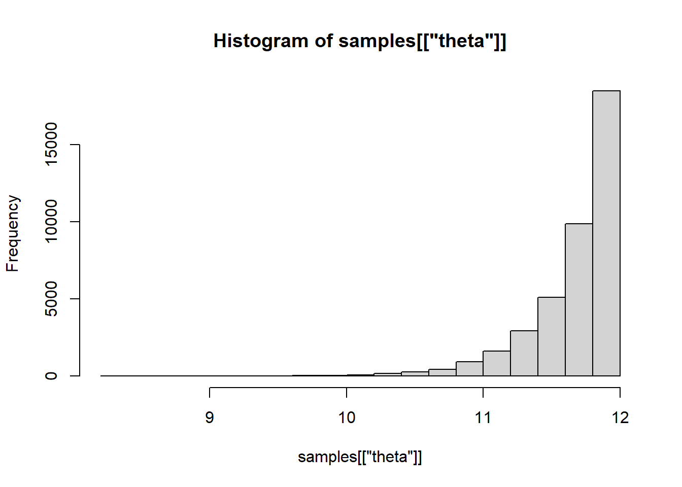
We can use R to access the samples from the model and plot the posterior probability density for \(\theta\) using a histogram.

params <- extract(fit)
samples <- tibble::as_tibble(params)

hist(samples[["theta"]])

Conclusion

We can use the samples generated from our Monte Carlo simulation to estimate the probability that \(\theta\) is between 11.23 and 12:

samples |>
    select(theta) |>
    count(11.23 < theta & theta < 12) |>
    mutate(prop = n / sum(n))
#> # A tibble: 2 × 3
#>   `11.23 < theta & theta < 12`     n  prop
#>   <lgl[1d]>                    <int> <dbl>
#> 1 FALSE                         4039 0.101
#> 2 TRUE                         35961 0.899

The results tell us that 89.9% of the simulated samples of \(\theta\) are in this range, which shows that 11.12 and 12 is a 90% credible interval for \(\theta\). We’ve managed to reproduce the result from the Jaynes paper!